5HAW
An old data scientist learning new tricks in 5 hours a week
Week 1: Reading data from a pdf using pdftools
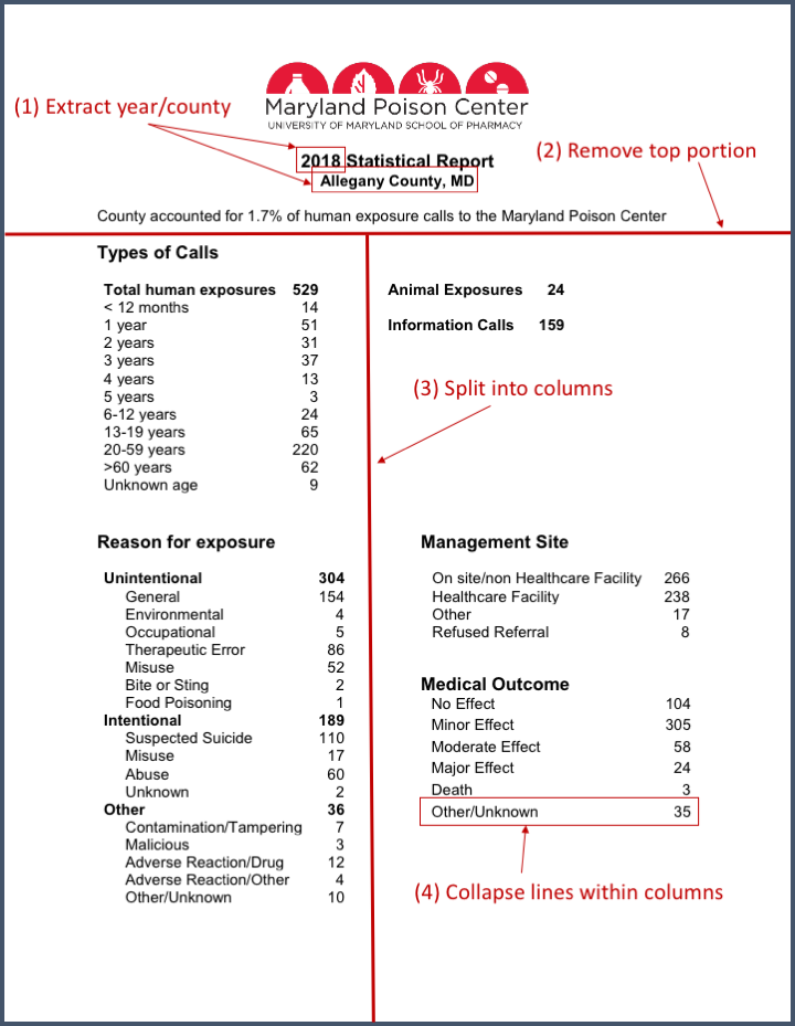
For week 1, I chose to tackle extracting data from a pdf document using the R package pdftools. My goal was to read in the data from the first page of this document, which gives exposure counts for calls to the Maryland Poison Center for Allegany County in 2018. Then I wanted to repeat this process for each county in Maryland for 2006-2018 and create a tidy and clean dataset of calls to the Maryland Poison Center (MPC). I am not exactly sure what I’ll do with the data once I’ve collected and cleaned it, but I think it might lend to some cool graphics of some type.
Here was my game plan:
- Extract the data from the Allegany County 2018 pdf document.
- After figuring it out for the Allegany County 2018 document, write a function to extract data from any pdf document with this structure (all MPC county reports have this same structure from 2006-2018)
- Test this function on two additional counties (Prince George’s County, Talbot County) for 2018; update function as needed.
- Download all 312 county pdf files (24 counties by 13 years) for 2006-2018.
- Attempt to extract data from all 312 pdfs, modifying the function as needed to handle any errors.
- Clean the resulting data set.
I managed to get through the first 5 steps and into the 6th before realizing it was going to take much more than 5 hours to complete this process; I pushed the completion of the project to Week2.
Time this week: 390 minutes (6.5 hours)
Total time: 746 minutes (~ 12.5 hours, ~ 6.25 hours/week)
I spent 6.5 hours on this project this week, with the time breakdown shown below. (As always, this time doesn’t include any blogging time about the project.)
| Mon 6.10 | Tue 6.11 | Wed 6.12 | Thu 6.13 | Fri 6.15 | Sat 6.15 | Sun 6.16 |
|---|---|---|---|---|---|---|
| 0 | 105 | 95 | 135 | 0 | 55 | 0 |
A stream of consciousness of my analysis process can be found here, and will be updated as I continue this project and eventually tidied after. Here are a few hightlights.
Reading in data from a single document: pdf_text vs pdf_data
Based on some simple googling, I knew that I wanted to use the pdftools package to extract the data. Many of the online examples used the pdf_text() function to read in lines of text from the pdf file, but then I found this information about doing low-level text extraction from a pdf using pdf_data() from an updated version of pdftools. Which one was the best one to use? I decided look at the result of each one. In each case, the function returns results separately for each page in the pdf document. Since I’m only interesting in extracting data from the first page of the document, I started by looking at how the first page looks with each function.
myData <- pdf_text("./data/Allegany County Statistical Report 2018.pdf")
myData[[1]]
## [1] " 2018 Statistical Report\n Allegany County, MD\nCounty accounted for 1.7% of human exposure calls to the Maryland Poison Center\nTypes of Calls\n Total human exposures 529 Animal Exposures 24\n < 12 months 14\n 1 year 51 Information Calls 159\n 2 years 31\n 3 years 37\n 4 years 13\n 5 years 3\n 6-12 years 24\n 13-19 years 65\n 20-59 years 220\n >60 years 62\n Unknown age 9\nReason for exposure Management Site\n Unintentional 304 On site/non Healthcare Facility 266\n General 154 Healthcare Facility 238\n Environmental 4 Other 17\n Occupational 5 Refused Referral 8\n Therapeutic Error 86\n Misuse 52\n Bite or Sting 2 Medical Outcome\n Food Poisoning 1 No Effect 104\n Intentional 189 Minor Effect 305\n Suspected Suicide 110\n Moderate Effect 58\n Misuse 17\n Abuse 60 Major Effect 24\n Unknown 2 Death 3\n Other 36 Other/Unknown 35\n Contamination/Tampering 7\n Malicious 3\n Adverse Reaction/Drug 12\n Adverse Reaction/Other 4\n Other/Unknown 10\n"With pdf_text(), we get one long element containing all of the text on the entire page, interspersed with newline characters (\n). If I use this function to extract the data, I will have to split on the newline character in order to separate the rows of data.
myData2 <- pdf_data("./data/Allegany County Statistical Report 2018.pdf")
myData2[[1]]
## # A tibble: 147 x 6
## width height x y space text
## <int> <int> <int> <int> <lgl> <chr>
## 1 31 12 230 116 TRUE 2018
## 2 66 12 266 116 TRUE Statistical
## 3 44 12 336 116 FALSE Report
## 4 50 11 246 132 TRUE Allegany
## 5 44 11 299 132 TRUE County,
## 6 18 11 347 132 FALSE MD
## 7 38 11 72 159 TRUE County
## 8 55 11 113 159 TRUE accounted
## 9 14 11 172 159 TRUE for
## 10 27 11 189 159 TRUE 1.7%
## # … with 137 more rowsWith pdf_data(), each individual word/number has its own line in the data, with associated (x,y) values to designate the text’s starting location. This means I can keep texts from the same line together by pulling text with the same y-value together. But, beyond this, I can also separate the columns of the data by using the x-value, which is helpful because parts of the document have two pieces of data on the same line.
You can see what I mean here, where I collapse the text within the same line together based on x values:
pdfData <- pdf_data("./data/Allegany County Statistical Report 2018.pdf")
p1Data <- pdfData[[1]]

p1Data %>%
  group_by(y) %>%
  arrange(x, .by_group=TRUE) %>%
  summarize(line = paste(text, collapse=" "))
## # A tibble: 43 x 2
## y line
## <int> <chr>
## 1 116 2018 Statistical Report
## 2 132 Allegany County, MD
## 3 159 County accounted for 1.7% of human exposure calls to the Maryland Poison Center
## 4 187 Types of Calls
## 5 217 Total human exposures 529 Animal Exposures 24
## 6 231 < 12 months 14
## 7 244 1 year 51 Information Calls 159
## 8 258 2 years 31
## 9 272 3 years 37
## 10 286 4 years 13
## # … with 33 more rowsIn line 5, there are two separate pieces of information: The total number of human exposures was 529 and the number of animal exposures was 24. I want to be able to easily separate these two pieces of information; I can do that by using the y-values for each piece of text to divide the text pieces into two columns.
I can also see that the first few lines of text don’t contain any data, but do contain the year and county for the document. Taking this into account, my strategy became:
- Extract the year and county from the first three lines of the data
- Remove these first three lines
- Divide the remaining text into two columns
- Collapse the text into lines separately within each column
Here’s a picture of this plan:
First, I extract the year and county by ordering the data by the y and x values and then selecting the relevant pieces:
orderedData <- p1Data %>% arrange(y,x)
orderedData
## # A tibble: 147 x 6
## width height x y space text
## <int> <int> <int> <int> <lgl> <chr>
## 1 31 12 230 116 TRUE 2018
## 2 66 12 266 116 TRUE Statistical
## 3 44 12 336 116 FALSE Report
## 4 50 11 246 132 TRUE Allegany
## 5 44 11 299 132 TRUE County,
## 6 18 11 347 132 FALSE MD
## 7 38 11 72 159 TRUE County
## 8 55 11 113 159 TRUE accounted
## 9 14 11 172 159 TRUE for
## 10 27 11 189 159 TRUE 1.7%
## # … with 137 more rowsyear <- orderedData$text[1]
county <- paste(orderedData$text[4:5],collapse=" ")
county = gsub(",","",county)
county; year## [1] "Allegany County"## [1] "2018"Next, I remove these first three header rows and then split into two columns. To do this, I see that the first three rows of data end at y=159 and the fourth row starts at y=187, so I can filter on y > 160 to remove these rows.
p1Data %>% group_by(y) %>% summarize(n=n())## # A tibble: 43 x 2
## y n
## <int> <int>
## 1 116 3
## 2 132 3
## 3 159 13
## 4 187 3
## 5 217 7
## 6 231 4
## 7 244 6
## 8 258 3
## 9 272 3
## 10 286 3
## # … with 33 more rowsp1Data <- p1Data %>% filter(y > 160)Now I can split the data into two groups by columns. To find where the column break is, I look at the x values for the text 7 (from the first column) and the text Animal (from the second column)
p1Data %>% filter(text=="7" | text=="Animal")## # A tibble: 2 x 6
## width height x y space text
## <int> <int> <int> <int> <lgl> <chr>
## 1 39 11 298 217 TRUE Animal
## 2 6 11 258 635 FALSE 7I can see that the end of the first column is at x=258 and the start of the second column is at x=298, so I can split the columns by x < 260 and designate these two columns with a new column variable:
p1Data <- p1Data %>%
  mutate(column=ifelse(x < 260, "Left", "Right"))
Finally, I can collapse lines within a column by first grouping by column, then grouping by y and collapsing across x:
lineData <- p1Data %>%
  group_by(column,y) %>%
  arrange(x, .by_group=TRUE) %>%
  summarize(line = paste(text, collapse=" "))

lineData
## # A tibble: 47 x 3
## # Groups: column [2]
## column y line
## <chr> <int> <chr>
## 1 Left 187 Types of Calls
## 2 Left 217 Total human exposures 529
## 3 Left 231 < 12 months 14
## 4 Left 244 1 year 51
## 5 Left 258 2 years 31
## 6 Left 272 3 years 37
## 7 Left 286 4 years 13
## 8 Left 300 5 years 3
## 9 Left 313 6-12 years 24
## 10 Left 327 13-19 years 65
## # … with 37 more rowsNow I don’t actually want to collapse across all text in a row, because the last text value is the count of observations in that category. So I want to keep the last text piece as the variable’s value and then use the previous pieces to make up the variable’s name. Once I label these pieces appropriately, I can collapse across the values of the variable’s name to get both the variable itself and the count for that variable.
groupedData <- p1Data %>%
  group_by(column,y) %>%
  arrange(x, .by_group=TRUE) %>%
  mutate(type = ifelse(x==max(x), "value", "name"))

groupedData
## # A tibble: 128 x 8
## # Groups: column, y [47]
## width height x y space text column type
## <int> <int> <int> <int> <lgl> <chr> <chr> <chr>
## 1 40 12 72 187 TRUE Types Left name
## 2 13 12 116 187 TRUE of Left name
## 3 33 12 133 187 FALSE Calls Left value
## 4 28 11 77 217 TRUE Total Left name
## 5 39 11 109 217 TRUE human Left name
## 6 59 11 152 217 FALSE exposures Left name
## 7 20 11 224 217 FALSE 529 Left value
## 8 7 11 77 231 TRUE < Left name
## 9 13 11 87 231 TRUE 12 Left name
## 10 39 11 104 231 FALSE months Left name
## # … with 118 more rowscountData <- groupedData %>%
group_by(column, y) %>%
arrange(x, .by_group=TRUE) %>%
summarize(variable = paste(text[type=="name"], collapse=" "), count=text[type=="value"])
countData## # A tibble: 47 x 4
## # Groups: column [2]
## column y variable count
## <chr> <int> <chr> <chr>
## 1 Left 187 Types of Calls
## 2 Left 217 Total human exposures 529
## 3 Left 231 < 12 months 14
## 4 Left 244 1 year 51
## 5 Left 258 2 years 31
## 6 Left 272 3 years 37
## 7 Left 286 4 years 13
## 8 Left 300 5 years 3
## 9 Left 313 6-12 years 24
## 10 Left 327 13-19 years 65
## # … with 37 more rowsFinally, I see there are some lines that are just text and not variables/counts, like “Types of Calls”, so I just remove them:
countData <- countData %>% filter(count != "Calls", count!="exposure", count!="Site", count!="Outcome")And then pull the variables/counts together into a data frame:
myRow <- as.data.frame(t(as.numeric(countData$count)))
names(myRow) <- countData$variable
myRow$Year <- year
myRow$County <- county
Testing my process on two additional documents
At this point, based on what I had done so far, I created a function that takes a pdf document and returns a data frame with a row of data for that pdf. I then tested this function of two additional documents, for Prince George’s (PG) County 2018 and Talbot County 2018. My function failed for both of these new documents because:
- The pdf document for Prince George’s County has an additional note at the top that reads “NOTE: This report reflects only the calls to the Maryland Poison Center from Prince Georges County. For complete statistics regarding Prince Georges County, statistics from the National Capitol Poison Center should also be consulted.” This is true for all years of data for PG County and also for Montgomery County. This throws off the removal of the top portion of the document, which I’ve set to be just the first 3 lines of data.
- For Talbot County, the text is shifted slightly down on the page so that the initial three lines end at the point
y = 164(noty = 159like for my original Allegany County document). This also throws off the removal of the top portion of the document. - The county name for PG County has three words (“Prince Georges County”), not two like the original document (“Allegany County”), which is problematic for how I select the county name. There are many other Maryland counties with three words as well.
My solution for the first two issues was to not hard code a cut at y > 160 to remove the top portion of the document and instead to cut after the 3rd line (whatever y-value that line may have) for all counties except for PG and Montgomery, which I will cut after the 6th line. I can do this with the following code:
if (county=="Prince Georges County" | county=="Montgomery County") {
  y.cut <- p1Data %>% group_by(y) %>% arrange(y) %>% summarize(n=n()) %>%
    slice(6) %>% select(y) %>% as.numeric()
  p1Data <- p1Data %>% filter(y > y.cut + 1)
} else {
  y.cut <- p1Data %>% group_by(y) %>% arrange(y) %>% summarize(n=n()) %>%
    slice(3) %>% select(y) %>% as.numeric()
  p1Data <- p1Data %>% filter(y > y.cut + 1)
}
My solution for the last issue was to just collapse the whole line to get the county name, since this will work regardless of the number of words that make up the county name. This means that I will have “Allegany County, MD” instead of just “Allegany County”, but this is fine with me. Here’s the new code to extract county/year:
year <- p1Data %>% arrange(y,x) %>% slice(1) %>% select(text) %>% as.numeric()

county <- p1Data %>% group_by(y) %>%
  arrange(x, .by_group=TRUE) %>%
  summarize(line = paste(text, collapse=" ")) %>%
  slice(2) %>% select(line) %>% as.character()
Downloading all pdf documents
With my function working on three of the files, it was time to download all of the pdf documents from the web. This was straightforward, since all of the URLs have the same format, except for those from 2016, which I could easily account for separately.
First I set up the counties and years I wanted:
countyNames <- c("Allegany County", "Anne Arundel County", "Baltimore City", "Baltimore County", "Calvert County", "Caroline County", "Carroll County", "Cecil County", "Charles County", "Dorchester County", "Frederick County", "Garrett County", "Harford County", "Howard County", "Kent County", "Montgomery County", "Prince Georges County", "Queen Annes County", "Somerset County", "St Marys County", "Talbot County", "Washington County", "Wicomico County", "Worcester County")

years <- 2006:2018
Then I created a link for each county/year combination as well as a file name where the downloaded file would be stored:
links <- NULL
files <- NULL
for (i in years) {
  for (j in countyNames) {
    countyNameForLink <- paste(unlist(strsplit(j, " ")), collapse="%20")
    if (i != 2016) {
      tempLink <- paste0("https://www.mdpoison.com/media/SOP/mdpoisoncom/factsandreports/reports/countypdf",i,"/",countyNameForLink,"%20Statistical%20Report%20",i,".pdf")} else {
      tempLink <- paste0("https://www.mdpoison.com/media/SOP/mdpoisoncom/factsandreports/reports/county-pdf-",i,"/",countyNameForLink,"%20Statistical%20Report%20",i,".pdf")}
    tempFile <- paste0(j," Statistical Report ", i,".pdf")
    links <- c(links, tempLink)
    files <- c(files, tempFile)
  }
}
After testing, I was able to download and save them all at once:
length(links)
for (i in 1:length(links)) {
  download.file(links[i], paste0("./data/",files[i]))
}
Processing all pdf documents with data extraction function
With the documents downloaded, I was hopeful it would be a simple matter to run each pdf document through my function (pdfMPC.page1()) and then bind the data from each document together. The code below will do this; note that the options(warn=2) function allows the warnings to be shown in the middle of the for loop instead of all at the end.
d1 <- pdfMPC.page1(paste0("./data/",files[1]))
myData <- d1

options(warn=2)
for (i in 2:length(files)) {
  di <- pdfMPC.page1(paste0("./data/",files[i]))
  myData <- bind_rows(myData,di)
  print(i)
}
Of course, it didn’t work perfectly the first time! Instead there were various warnings/errors that had to be addressed for particular files. In particular, I had to update my function to deal with:
- Removing commas from counts, for example changing 5,321 to 5321. (Baltimore County 2006 and others)
- Accounting for blank counts where the row had a name but not a value; I set these counts to 0. (Somerset County 2006 and others)
- Removing “Maryland Poison Center” printed across the bottom of page 1 for come counties/years. (Cecil County 2007 and others)
- Handling apostrophes in two county names that caused one line of code to be recognized as two, meaning the header needed to be removed after 4 lines instead of 3. (Queen Anne’s County 2011, St Mary’s County 2011 and other years)
After making these modifications, I was finally left with a function that would work for all 312 of the pdf files!
pdfMPC.page1 <- function(pdf.file) {
  require(dplyr)
  require(pdftools)

# read in the pdf document; select the first page
pdfData <- pdf_data(pdf.file)
p1Data <- pdfData[[1]]

# get the year and country from the header
year <- p1Data %>% arrange(y,x) %>% slice(1) %>% select(text) %>% as.numeric()

county <- p1Data %>% group_by(y) %>%
  arrange(x, .by_group=TRUE) %>%
  summarize(line = paste(text, collapse=" ")) %>%
  slice(2) %>% select(line) %>% as.character()

# remove the header
# the first 3 lines for most, the first 6 lines for PG and M counties
if (county=="Prince Georges County, MD" | county=="Montgomery County, MD") {
  y.cut <- p1Data %>% group_by(y) %>% arrange(y) %>% summarize(n=n()) %>%
    slice(6) %>% select(y) %>% as.numeric()
  p1Data <- p1Data %>% filter(y > y.cut + 1)
} else {
  if (county=="Queen Anne’s" | county=="St. Mary’s") {
      y.cut <- p1Data %>% group_by(y) %>% arrange(y) %>% summarize(n=n()) %>%
    slice(4) %>% select(y) %>% as.numeric()
  p1Data <- p1Data %>% filter(y > y.cut + 1)
  county <- paste0(county," County, MD")
  } else {
    y.cut <- p1Data %>% group_by(y) %>% arrange(y) %>%
      summarize(n=n()) %>%
      slice(3) %>% select(y) %>% as.numeric()
    p1Data <- p1Data %>% filter(y > y.cut + 1)
  }
}

# create the column variable (Left/Right)
p1Data <- p1Data %>%
  mutate(column=ifelse(x < 265, "Left", "Right"))

# group the data by column and height on the page
# keep the last entry of that column/height as the value
# assign the remaining entries for that column/height the name
groupedData <- p1Data %>%
  group_by(column,y) %>%
  arrange(x, .by_group=TRUE) %>%
  mutate(type = ifelse(x==max(x) & x==min(x), "name", ifelse(x==max(x), "value", "name")))

# collapse the entries for name together to create the variable name
# keep the value as the count
countData <- groupedData %>%
  group_by(column, y) %>%
  arrange(x, .by_group=TRUE) %>%
  summarize(variable = paste(text[type=="name"], collapse=" "), count=ifelse(is_empty(text[type=="value"])==FALSE, text[type=="value"],"0"))

# remove the rows that aren't variables/counts
countData <- countData %>% filter(count != "Calls", count!="exposure", count!="Site", count!="Outcome", count!="Center", variable!="Maryland")

# create the data frame for this county/date
myRow <- as.data.frame(t(as.numeric(gsub(",","",countData$count))))
names(myRow) <- countData$variable
myRow$Year <- year
myRow$County <- county

return(myRow)
}
Althought I now had a data frame with 312 rows, one for each county/year combination, there was still much work to be done in the form of data cleaning. This was the project for Week 2!
[How did I discover this data in the first place? I’ve thankfully never had to call MPC for my children, but did call them late one night when, in the sleep-deprived state of having a newborn, I accidently took two Claritin instead of one and then panicked because I didn’t know if I should still nurse my child. A very kind pharmacist allayed my fears and pointed me to parental references on their website, and that’s when I discovered all this county-level data tied up in pdf files. I had always intended to try to do something with this data, and now I finally am.]